How to Color Alternate Rows or Columns in MS Excel

An Excel sheet can quickly get cluttered with lots of data. And, in the plain black and white format it can get difficult to follow the rows and the data in them. One of the best ways to make things clearer is to color every alternate row in the sheet.

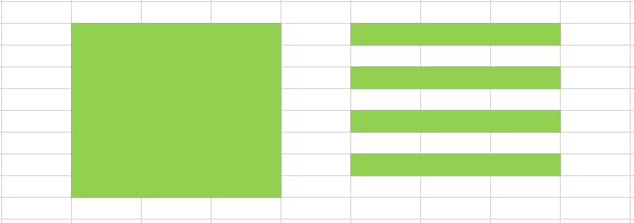
Some people like to highlight a block of data to make it distinct from the rest. To me alternate highlighting is always better to the eyes than a complete colored block. See the difference below and if you like it, read on.

One can always convert the data into a table and choose from the numerous table formats. But, when you do that you import all table properties, that’s not always required. So, we will learn how to get alternate shading while leaving the table and table properties aside.

Note: The tutorial uses MS Excel 2010. However, the trick remains the same on all versions. Only the ribbon may vary a little.

Steps to Color Alternate Rows

We will apply some conditional formatting and a couple of formulas. I suggest that you should practice along. So, open an Excel sheet right away.

Step 1: Select the cells where you want to apply alternate shading. If you want to do it for the entire sheet, press Ctrl + A.

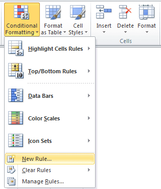
Step 2: Navigate to Home tab and select Conditional Formatting from under Styles section. Choose to create a New Rule.

Step 3: On the New Formatting Rule window Select a Rule Type– Use a formula to determine which cells to format.

Step 4: On Edit the Rule Description section enter the formula =mod(row(), 2)=0 and then click on Format.

Step 5: On the Format Cells window, switch to Fill tab, select your color and hit on Ok.

Step 6: Back to the Formatting Rule window you will get a preview of your formatting. Click on Ok if you are done with your selection.

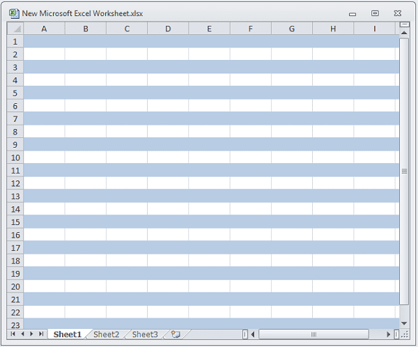
Here’s how I colored the entire sheet with alternate blue rows.

At any given time you can navigate to Conditional Formatting -> Manage Rules and edit the format attributes.

Cool Tip 1: Using the formula =mod(row(), 2)=0 will shade the even numbered rows. If you wish to shade the odd rows try =mod(row(), 2)=1.

Cool Tip 2: Want to alternate shading with two different colors? Create one rule with =mod(row(), 2)=0 and select a color. Create another rule with =mod(row(), 2)=1 and select another color.

Cool Tip 3: If you wish to color alternate columns instead of alternate rows you can use the same trick. Just replace row() by column().

If you noticed, when you fill the cells with colors they overlay the sheet gridlines. Unfortunately there is no way to bring them to the front. What you can do is apply borders to all cells, choose thin lines and color that’s close to the default gridlines color.

The closest match of the border and the gridlines color is the color index R:208 G:215 B:229.

Conclusion

That’s all about shading of alternate rows in Excel. Easy and interesting, right? Next time you find a sheet illegible, you have no reason to complain. All you need to do is spend a few minutes on formatting and you are done. And, make sure to present your data with good contrasts next time.

Photo Credit: sacks08