How to Color Alternate Rows or Columns in Google Sheets

Microsoft Office is a powerful tool to get things done, but Google isn’t all that far behind with its Google Docs offering. The latter is not only free, but also saves you a backup on the free app on Android and iOS devices.

While MS Office has some great features which are not easy to find in Google Docs, there are always solutions and workarounds to them. Most users have yet not figured out that you can get a striped table easily in Google Sheets, quite like the ‘Quick Styles’ menu in MS Office.

How to get that done, though? It’s quite simple.

The Magic Formula for Rows

The Google Docs suite doesn’t support zebra stripes directly, but the workaround is to use conditional formatting. Things have changed over the years, so it’ll be a bit harder to find it in its current avatar.

First, hit the Format option from the menu at the top and then click Conditional formatting. Once you do, you will see the below screen with a few options available to you.

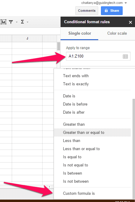
From here, select the range which you will need to work on. As an example, I’ve gone from A1 to Z100, but if you already know your specific range, then go with that. Next, click on Custom formula is which will bring you to the window below.

Type in the formula in the box waiting for your prompt, as is

=ISEVEN(ROW())

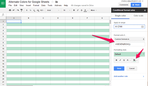
As soon as you enter the formula here, you will see the sheet turn in to a zebra. There will be alternate rows filled with the specified color that you’ve chosen and changing the color itself is as easy as clicking on the icon.

Once this is done, click on Add another rule and instead of the previous formula, insert this particular formula

=ISODD(ROW())

That’s the whole idea. Again, if you want to change the color, simply click on the corresponding icon and choose the look you want.

Same Formula Works for Columns

The same methodology also works for columns. But instead of using the ROW function in our above formula, we need to replace it with COLUMN. Specifically, =ISEVEN(COLUMN())

That’s it, all the previous steps are pretty much the same, including adding the formula for odd numbered columns too.

Everything on Google Drive: We’ve covered a myriad of topics on Google Drive, including how to transfer ownership in Drive, how to open Google Drive files from its website in desktop apps, and also compared it to Dropbox and SpiderOak.

Easy as You Like it

I hope that was useful for those of you who use Google Drive and Sheets on a regular basis. We at GuidingTech certainly do and simple hacks like these are life-savers. Join us in our forum if you have any questions or have better hacks than the one suggested here.